Statistical Anomaly Discovery Through Visualization
Written by: Shine Xu
I defended on April 19 in DEH Room 220. All my committee attended in person. Many friends came to support me. The room is a small room but a good size for discussion. I started my defense with a brief overview of my research.
Overview
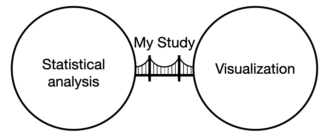
My study focuses on two fields: statistical analysis and visualization. My research explores various approaches to combine statistical analysis and visualization for discovering and examining anomalies in multidimensional data. For statistical analysis, my primary interest is statistical anomaly, specifically Simpson’s paradox and mix effects. My motivation is to discover instances of unfairness in data and to improve understanding of statistical anomalies.
Background
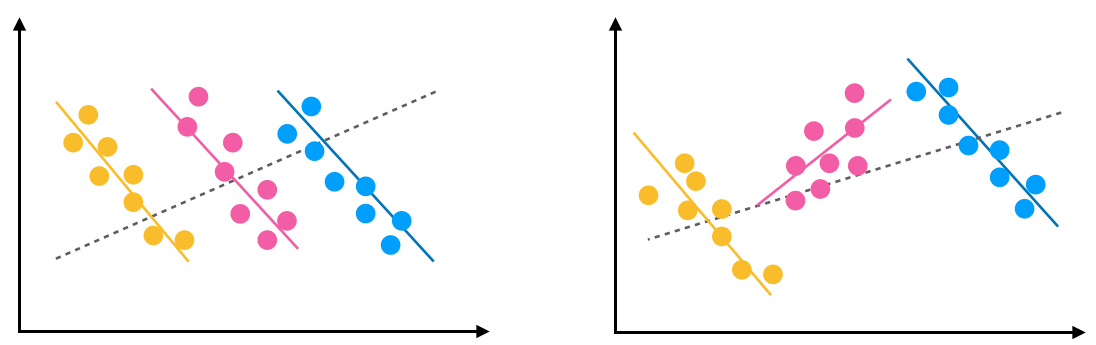
I studied two trends in data: regression trend and rank trend. A regression trend is a linear relationship between two variables. A rank trend is a ranking of groups defined by one variable according to a statistic calculated on a second variable. Trends in data can be misleading. However, we uncover some surprising trends when we split the data by another variable. When a trend between two variables is reversed in all subgroups of the data, it is Simpson’s paradox. If the trend is reversed for some subgroups, it is a “mix effect”.
Thesis
Combining composite visualizations for drill-down exploration with interactions into a visualization system supports effective comprehension and analysis of statistical anomalies in multidimensional data for the user with basic statistical knowledge. Adding capabilities to drill down into hierarchically dimensional combinations allows the user to visually observe correspondences between dimensional information. These capabilities allow users to readily discover statistical anomalies and explore their relationships in multidimensional data.
Research Path
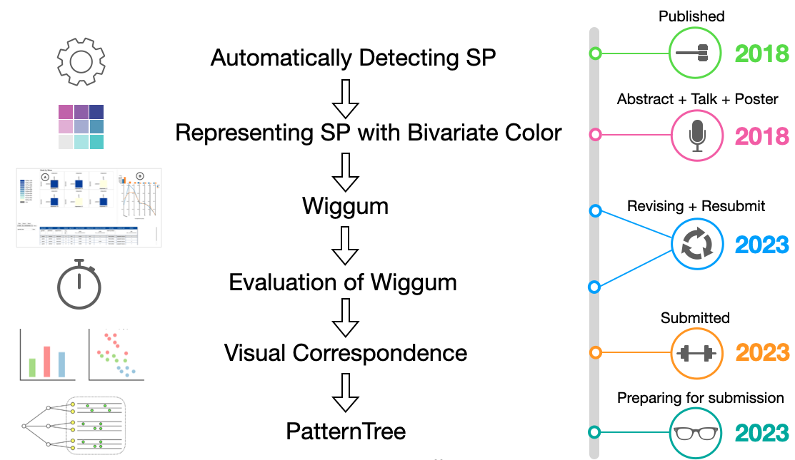
My research started by developing an algorithm for detecting regression trends for Simpson’s paradox. We published this work in 2018. Later, I explored visual techniques to represent Simpson’s paradox. I built a system called Wiggum to help users to detect and understand Simpson’s paradox and mix effects. And I performed a user study to evaluate the system. To improve Wiggum, I developed a model of visual correspondence for designers to consider correspondence in multi-view visualization. I also provided a PatternTree technique to embed views in a left-right node-link diagram.
Automatically Detecting Simpson’s Paradox
Method
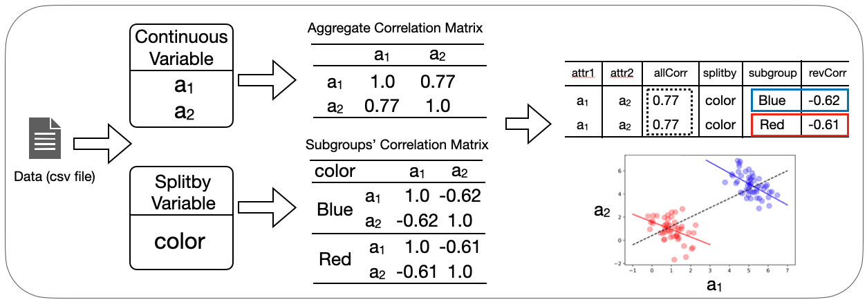
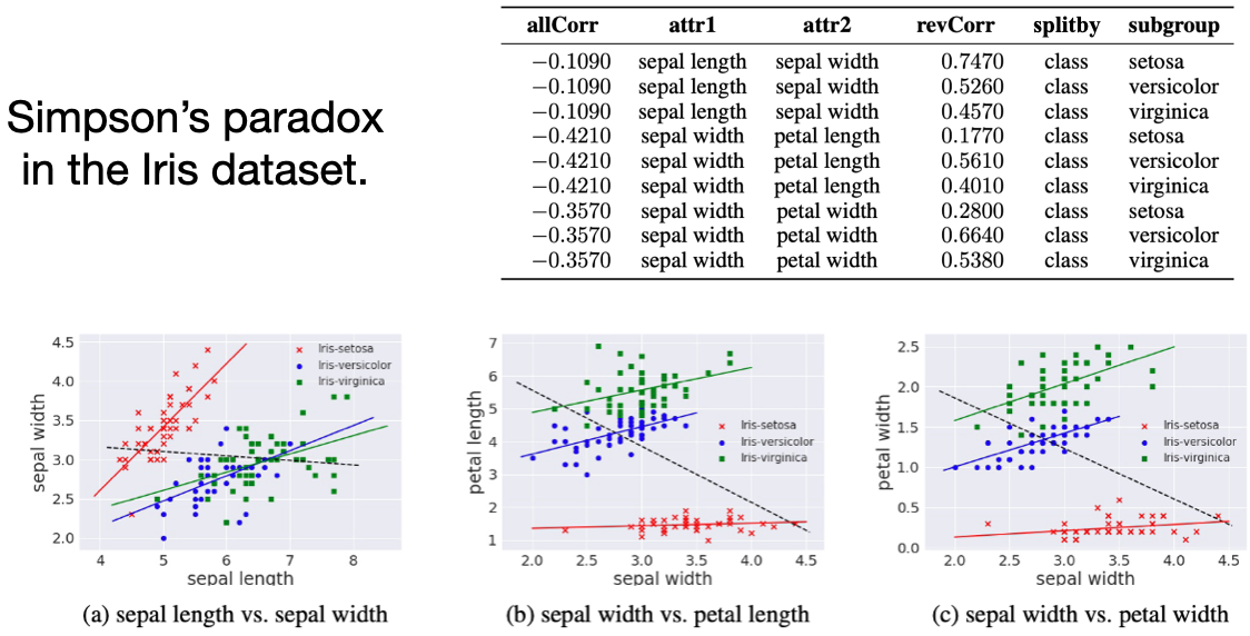
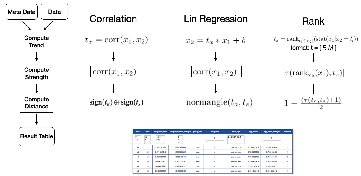
I use Pearson’s Correlation Coefficient to quantify the regression trend. After data is loaded, the attributes are categorized into two lists based on the attribute’s type. Then, the algorithm computes an aggregate correlation matrix by the continuous variable and a couple of subgroups’ correlation matrix of the data partitioned by a split by variable. Two types of matrices are combined to generate a result table. Each row in the result table shows an instance of the reverse trend.
Experiments
I applied my algorithm to the Iris dataset. We can observe Simpson’s paradox in the Iris dataset, since all subgroups show the reverse trend for a pair of continuous attributes.
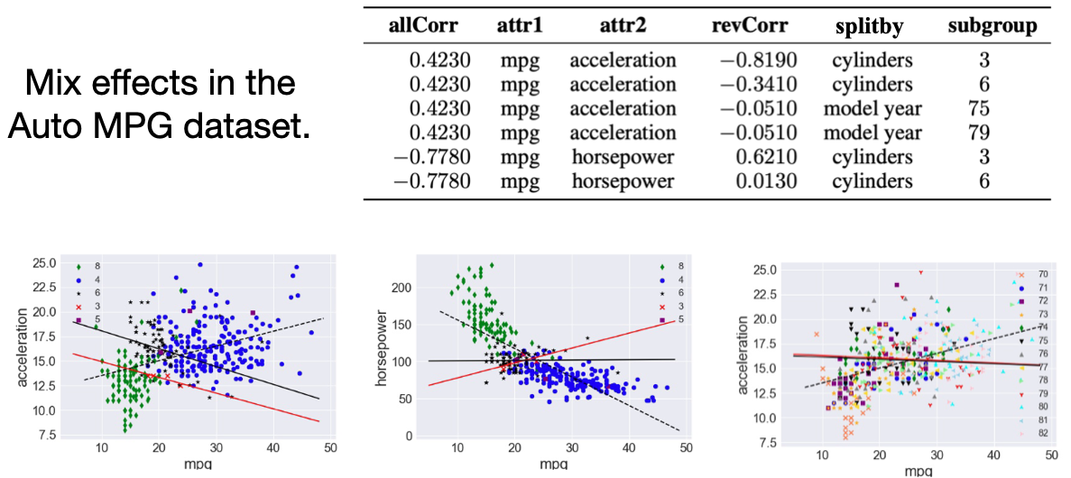
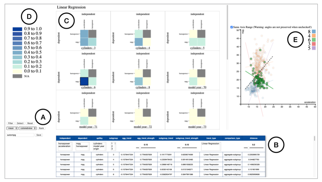
I also applied my algorithm to the Auto MPG dataset. In this dataset, we only can observe some mix effects. For example, only cylinder 3 and 6 show the reverse trend for acceleration vs. mpg.
Running Time of the Detection Algorithm
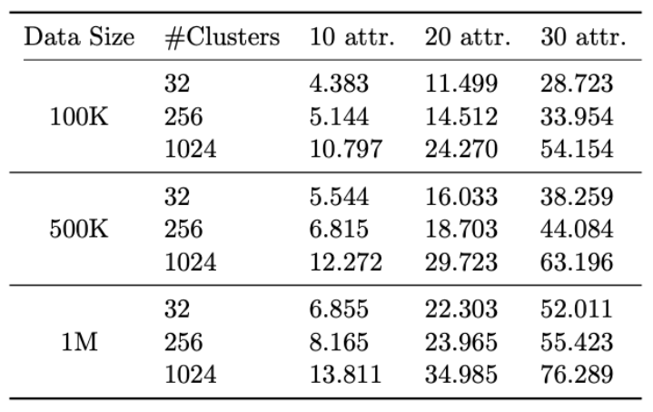
I measures the running time of my detection algorithm. I observe three important factors that make effect on running time: the total number of continous and split by attributes, the total number of records, and the levels for each split by attribute. We can precompute datasets quickly enough, and the computation will not impact interactive visualizations that I study.
Representing Simpson’s Paradox with Bivariate Colors
Encode Reverse Trend by Bivariate Color
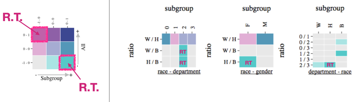
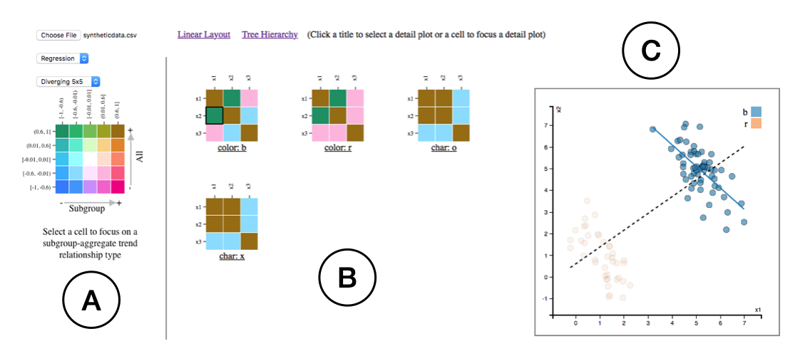
We can use a bivariate color scheme to represent reverse trend. The horizontal axis in the bivaraite color scheme indicates the subgroup statistic, and the vertical axis for aggregate statisic. As a result, the upper-right cell color and the bottom-right cell color indiate a reverse trend. We can look for those two colors in the heatmap overview to find reverse trend instances.
Apply Bivariate Color to Rank Trend
We applied the bivariate color to the rank trend. First, we can computer two ratios of summary statistics in terms of ranked groups for aggregate and subgroup data. The ratios indicate a relationship in rank trend. Then we use bivariate color to indicate the relationship between those two ratios.
![]()
Overview of Viusal Website
Our visualization web page consists of three parts. The left panel has a control panel and a legend. In the center, we provide an overview of all detected instances. In the right panel, a detail view is presented to help check the detail of the patterns.
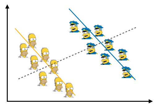
Wiggum
Wiggum is a fictional character from the animated television series The Simpsons; he is the police chief of Springfield. We use Wiggum to name our interactive visual analysis system which is used for revealing various forms of mix effects.
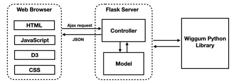
In the front end, we use D3 to draw views. In the back end, we develop a Wiggum Python Libray for all the computation tasks. We use Flask Server to connect and communicate between the front end and the back end.
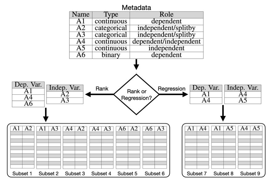
Generate Substets
Before performing computation, we need to generate subsets for measuring trends. Users need to set attributes’ roles and types, and the attributes’ information is stored in the metadata. We use the metadata to categorize the attributes by the rules in terms of trend types. For each trend type, there are always two lists of variables: dependent variable list and indenpendent varible list. The two lists are used to generate subsets by pairing different attributes in the lists.
Trend Measurements
After obtaining subsets, our system first compute trends based on subsets. Then it computes trend strength and trend distance. Different trend types have different computations. All the statistics will be stored in a result table.
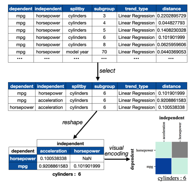
Generate Distance Heatmap
After we get the result table, we select a specific subgroup from the result table. We use the selection to reshape the selected data into a matrix like structure. We use color to encode the distance in the matrix. The distances for a specific subgroup can be visualized through the heatmap.
Auto MPG
This is an example for applying Wiggum to the Auto MPG dataset. In the center, we show an overview of all detected instances. The left side has a legend and a control panel. The bottom is a result table showing the detailed statistics. The right side is a detail view.
Evalation of Wiggum
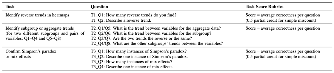
In the evaluation, we want to learn how well Wiggum helps users detect and understasnd mix effects. Our user study is a one-on-one Zoom meetings with participants. Participants are encouraged to think aloud and to ask questions. We have two pilot study participants and 37 main study participants.
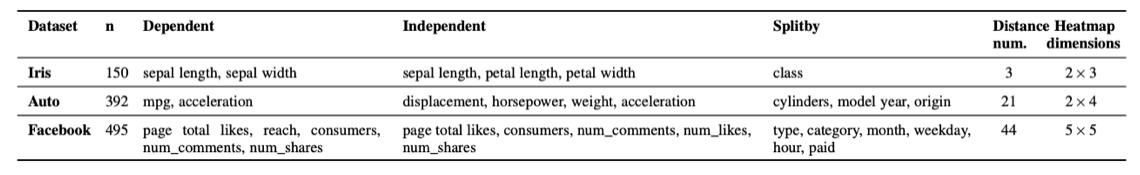
We used three datasets and designed tasks.
We plot the correctness versus tasks. From highlighted tasks, we observe that participants performed worse on the larger data sets.
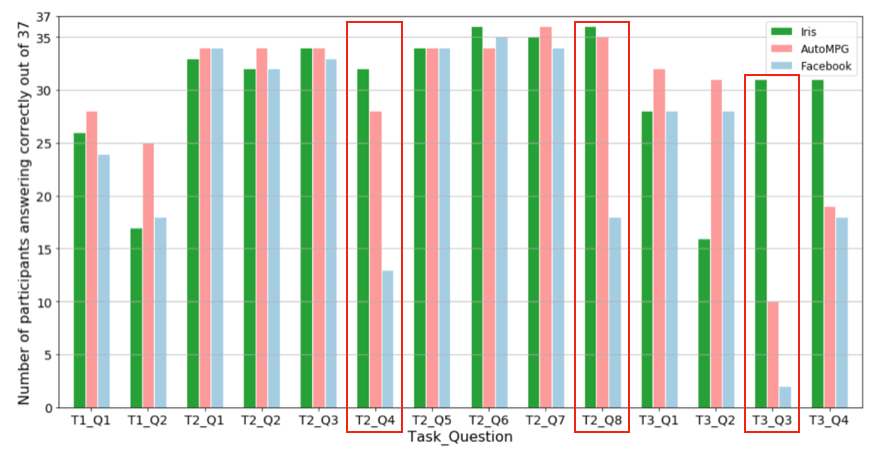
Overall we observe that Wiggum can help users understand the concept of mix effects. The structure of the information in the data becomes hard to perceive due to a combinatorial explosion of data dimensions. The variables conveying hierarchical information are crucial for users to perform tasks correctly and comprehend the relationship among variables.
Visual Correspondence
Complex visualizations often have different ways of showing the same information in different places.
We define visual correspondence as the extend to which visual encodings of the same or equivalent information are interpreted as being the same or equivalent.
We believe that developing a better theoretical understanding can help to have a better understanding about how to design multi-view visualizations.
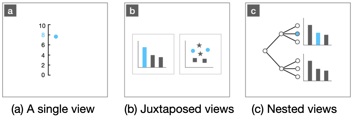
Three Basic Visual Designs for Considering Visual Correspondence
For visual correspondence, we consider three types of visual designs including a signle view, juxtaposed views and nested views. The graphical items in these three views could encode the same information data and correspond.
Degree of Correspondence
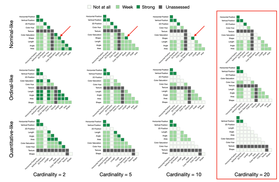
We measure the degree of correspondence by four factors: information aspect, a pair of visual channels, and cardinality. We use a lower diagonal matrix to represent all pairs of visual channels for a specific information aspect and a cardinality level. We design three cases to assess the visual correspondence for each pair of visual channel.
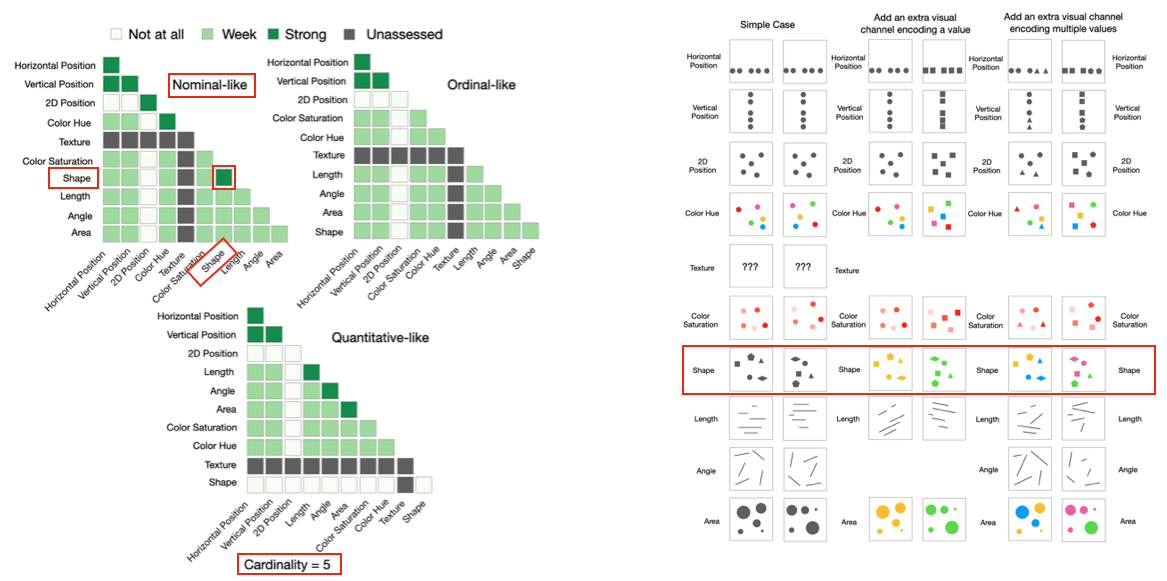
Populate the Combination Matrices
We apply our method to populate the combination matrices for for different cardinality levels. From the populated matrices, we can observe some interesting patterns. Cardinality is an important factor. When cardinality is 20, most pairs of visual channels can not generate strong visual correspondence. We also observe that same visual channel pairs work better.
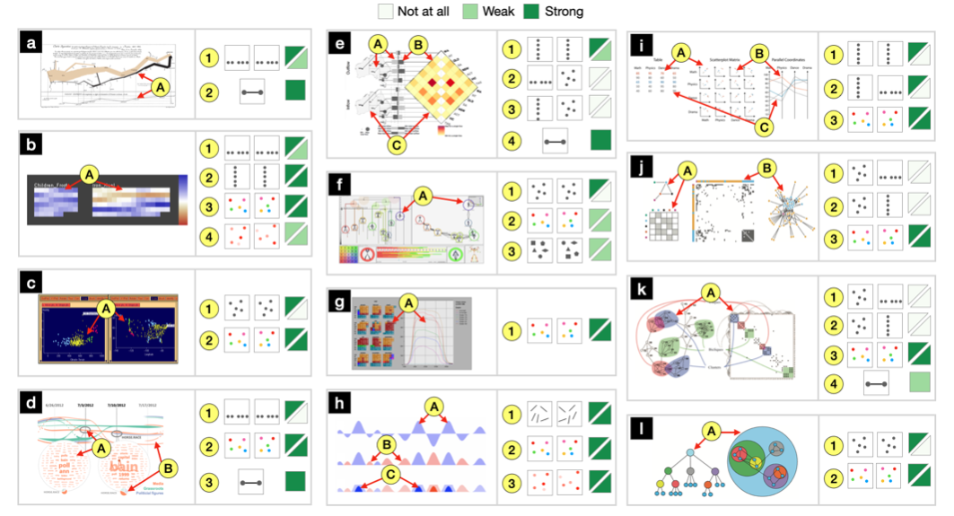
Applying the Result
We apply our populated matrices to 12 example visualizations. We compared the expected result with our predicted reuslt for visual correspondence. Some cases show the predictive power of the populated matrices from our model.
Guidelines
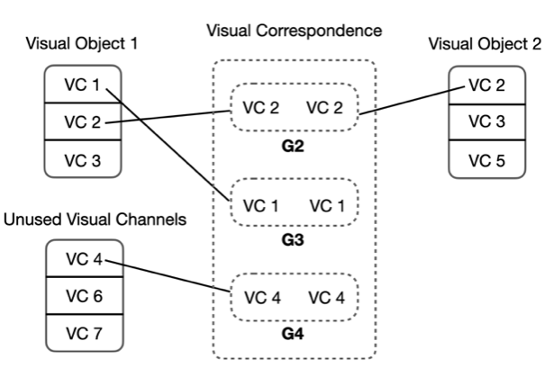
We propose a set of guidelines for designers who consider visual correspondence in multi-view visualization. G1: Consider more effective individual channels for corresponding visual objects. G2: If possible, choose the same or highly related visual channel for the corresponding visual objects. G3: If G2 fails, use the already used visual channel from one visual object. G4: If G2 and G3 fail, pick the most highly visual correspondent visual channel from unused visual channels.
We develop a model of visual correspondence to help associate graphical items which encode the same data through pairwise visual channels. We will apply our visual correspondence model to refine the design of PatternTree for revealing the relationship of graphical items between the host view and the embedded views.
PatternTree
We introduce PatternTree as hybrid tree visualization via a virtual layering technique to explore hierarchical patterns. We illustrate the usefulness of the features of our hierarchical pattern structure by applying it to the gerrymandering domain.
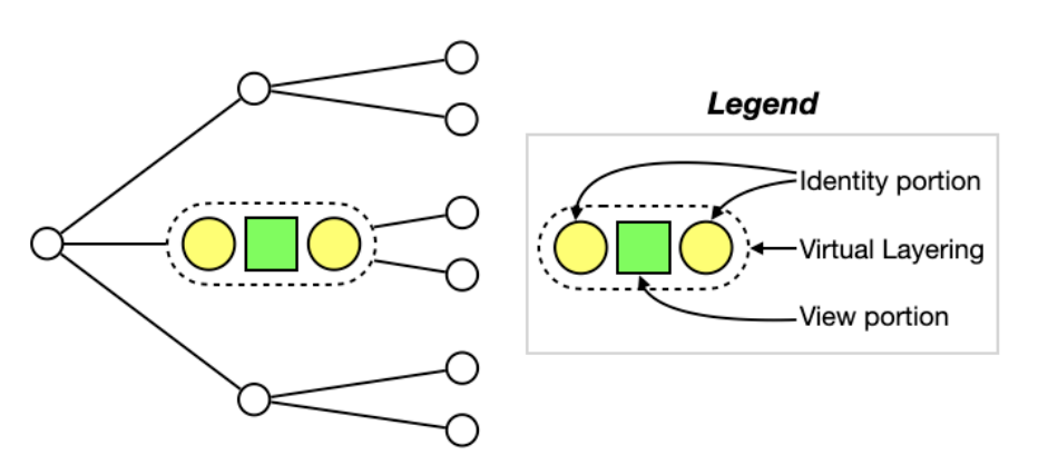
Virtual Layering
We propsed a technque called virtual layering. Virtual layering is a form of composite visualization that embeds multiple views as nodes inside a host node-link diagram. Virtual layering has identity potion and view potion. The identity portion indicate the level of node in the tree. The view potion is the embedded view.
Which Pattern is in Gerrymandering?
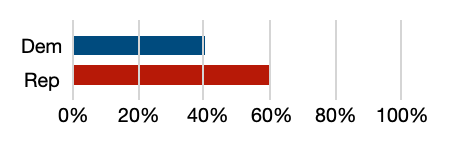
In gerrymandering, we cam computer voting share percentage for each party. If we compare two voting share percentages, it is similar to the rank trend.
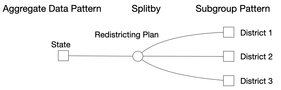
We can use the root node to represent the aggregate pattern which can be a state-level pattern. In the middle of the tree, we can use the middle nodes to represent the redistricting plans. And leaf nodes can represent districts’ patterns.
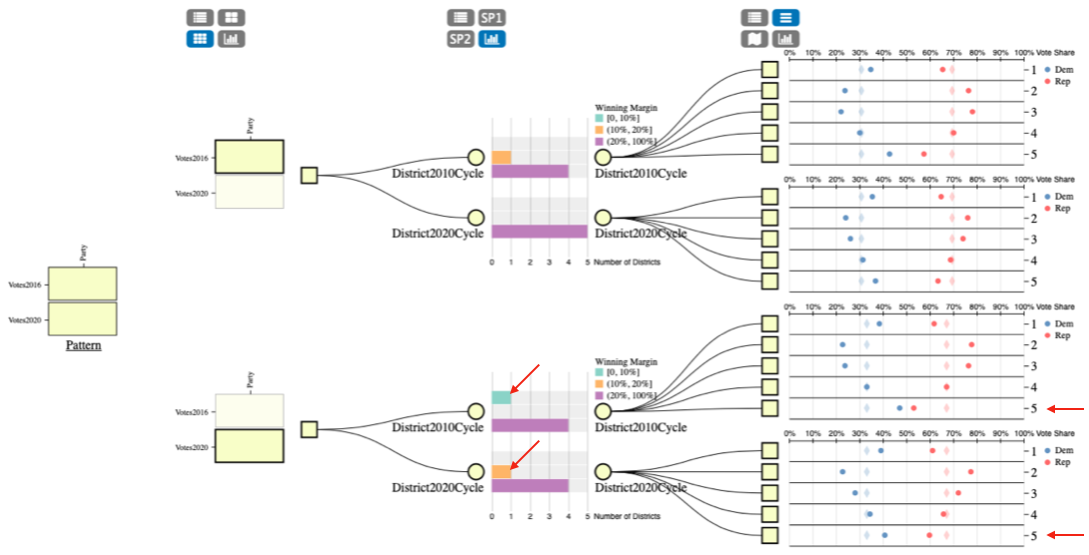
Assess the Electoral Competition
We design the PatternTree to assess the electoral competition for Oklahoma by 2016 and 2020 precidential voting data. It is easy to observe that in the lower branch a highly competitive district disappeared after redistricting plan while a moderately competetive district is shown after redistricting. We check a strip plot in the leaf node. We can confirm that district 5 used to be a highly competitive district but the difference between two parties’ voting share percentages becomes large after redistricting. Our findings in Oklahoma is a strong sign that gerrymandering can occur even without overturning the election.
Contribution
- A Python library of statistical computations and methods for detecting mix effects.
- A conceptual model for associating visual items encoding the same data by pairwise visual channels.
- A set of design guidelines for establishing and evaluating visual correspondence.
- A design space for embedding views in a node-link tree visualization for smooth visual transitions.
- View designs for understanding and efficiently detecting mix effects.
- An implementation of a visual analysis application, Wiggum.
- An evaluation of users’ ability to comprehend and apply statistical concepts in the user interface.
Future Work
- Apply Wiggum more broadly to meaningful real world problems.
- Explore other tree layouts for designing hybrid tree visualizations to reveal hierarchical patterns.
- Apply visual correspondence to other graph-structured data and visualizations.
- Perform user study on how people perceive visual correspondence.
Conclusion
The principle goal of this dissertation has been to develop and assess a visual analysis system approach in which complex statistical capabilities can be accessible to wider groups of users with a basic knowledge of statistics. The contributions in this work validate the effectiveness of the detection for statistical anomalies by demonstrating learnability, flexibility, and general applicability of the statistical methods for exploratory data analysis. This work opens up myriad of directions for future research on the way to greater data democratization.